An O'Raifeartaigh model and its Goldstino

A scalar direction can be flat even though its vacuum breaks supersymmetry. Does a massless fermion then require the scalar to remain massless? We will find both modes in one classical model and calculate the quantum correction that separates them.

This lesson continues the vacuum tests and the first quantum correction. We work in flat four-dimensional global $\mathcal N=1$ supersymmetry, with all four real supercharges manifest in the usual superspace. There are three neutral chiral multiplets, no gauge group and no supergravity. The calculation concerns constant scalar backgrounds and their fluctuations.

A model whose F equations cannot all vanish

Let $X,\phi_1,\phi_2$ denote chiral superfields and, when writing the potential, their scalar components. Choose

$$K=\bar X X+\bar\phi_1\phi_1+\bar\phi_2\phi_2,\qquad W=fX+\frac h2X\phi_1^2+m\phi_1\phi_2.$$

The fields have engineering dimension one; $f$ has dimension two, $m$ dimension one and $h$ dimension zero. Take all three coefficients nonzero. Independent constant rephasings of the fields allow us to choose $f,h,m>0$ for this calculation.

Write $W_i=\partial W/\partial\phi_i$, including $X$ among the fields. The canonical auxiliary equation is $F_i=-\overline{W_i}$. Here

$$W_X=f+\frac h2\phi_1^2,\qquad W_1=hX\phi_1+m\phi_2,\qquad W_2=m\phi_1.$$

If all auxiliaries vanished, $W_2=0$ would require $\phi_1=0$, but then $W_X=f\ne0$. There is no supersymmetric solution at a finite field value. That observation alone would not exclude an unstable stationary point or a runaway. We must inspect the potential:

$$V=\left|f+\frac h2\phi_1^2\right|^2 +|hX\phi_1+m\phi_2|^2+m^2|\phi_1|^2.$$

Define the dimensionless ratio

$$r=\frac{hf}{m^2},\qquad 0<r<1.$$

This restriction has a physical purpose. Since $\operatorname{Re}(\phi_1^2)\ge-|\phi_1|^2$,

$$V\ge f^2+(m^2-hf)|\phi_1|^2 +\frac{h^2}{4}|\phi_1|^4+|hX\phi_1+m\phi_2|^2.$$

Every term after $f^2$ is nonnegative. In the stated strict inequality, equality requires

$$\phi_1=\phi_2=0,\qquad X\ \text{arbitrary},\qquad V_{\rm tree}=f^2.$$

Thus we have found the full global classical minimum set, not just a stationary point. There is no classical direction with energy below $f^2$, even at arbitrarily large fields. Along the minimum set, $F_X=-f$ and the other auxiliaries vanish.

The complex coordinate $X$ is a pseudomodulus: a flat classical direction through nonsupersymmetric minima. Unlike a protected moduli space of supersymmetric vacua, this degeneracy can be lifted by quantum corrections. This is the canonical model of Intriligator–Seiberg, §2.5, (2.28)–(2.30).

Which massless particle is protected?

First expand about $X=\phi_1=\phi_2=0$. Use canonically normalized real fields, $\phi_1=(a+ib)/\sqrt2$ and $\phi_2=(c+id)/\sqrt2$. The quadratic potential is

$$V=f^2+\frac12(m^2+hf)a^2+\frac12(m^2-hf)b^2 +\frac12m^2(c^2+d^2)+\cdots.$$

The scalar $X$ supplies two additional real fields with zero tree-level mass. The fermion mass term is $-\tfrac12W_{ij}\psi_i\psi_j+\text{h.c.}$; at this point

$$W_{ij}= \begin{pmatrix} 0&0&0\\ 0&0&m\\ 0&m&0 \end{pmatrix}_{(X,1,2)}.$$

Hence $\psi_1,\psi_2$ form a massive pair with mass $m$, while $\psi_X$ is massless. The bosonic and fermionic masses have split:

Fluctuations	Squared masses at the origin
Two real components of $\phi_1$	$m^2+hf,\ m^2-hf$
Two real components of $\phi_2$	$m^2,\ m^2$
Two heavy Weyl fermions	$m^2,\ m^2$
Two real components of $X$ and the Weyl fermion $\psi_X$	$0,\ 0$ and $0$ at tree level

The fermion $\psi_X$ is the Goldstino, the massless fermionic mode associated with spontaneous breaking of global supersymmetry. At a constant bosonic background its transformation contains

$$\delta\psi_X=\sqrt2\,\epsilon F_X=-\sqrt2\,f\epsilon.$$

Its nonzero field-independent shift identifies the broken transformation. The massless direction can also be derived from stationarity. For canonical kinetic terms,

$$0=\partial_i V=W_{ij}\overline{W_j}.$$

Thus a nonzero F expectation value gives a null vector of the fermion mass matrix. In this model that vector points entirely along $X$.

The corresponding quantum Goldstino statement follows from the conserved supersymmetry current and its Ward identity in a regular vacuum with broken global supersymmetry. In infinite volume one formulates it using the current, rather than assuming that the broken charge creates a normalizable zero-momentum state. See Tong, §3.4.1. No such Ward identity requires the scalar partner to stay massless: the vacuum no longer organizes excitations into degenerate unbroken-supermultiplet spectra.

There is also an R symmetry with $R(X)=R(\phi_2)=2$ and $R(\phi_1)=0$, with the coefficients held fixed. At $X=0$ it is unbroken. The scalar flat direction there is therefore not a Goldstone boson of a broken R symmetry.

Keep the masses as functions of the background

A loop can lift $X$ only if the particles circulating in it feel $X$. Choose a point on the classical valley, $\phi_1=\phi_2=0$. The R symmetry rotates its phase, so we may use a real background $X=x$ to compute a potential that depends on $|X|$.

The heavy fermion mass matrix and its squared-mass matrix are

$$M_F(x)= \begin{pmatrix}hx&m\\m&0\end{pmatrix}, \qquad A(x)=M_F^\dagger M_F =\begin{pmatrix}m^2+h^2x^2&hmx\\hmx&m^2\end{pmatrix}.$$

Expanding the original scalar potential to quadratic order gives two real blocks. The $(a,c)$ block and $(b,d)$ block are respectively

$$B_+(x)=A(x)+hfP,\qquad B_-(x)=A(x)-hfP,\qquad P=\begin{pmatrix}1&0\\0&0\end{pmatrix}.$$

The term $fh\,\operatorname{Re}\phi_1^2$ causes the opposite shifts. These are mass-squared matrices: each $B$ has two real scalar eigenvalues, while $A$ has two Weyl-fermion mass-squared eigenvalues.

For $r<1$, both blocks are positive at every finite real $x$. For example their upper-left entries are positive and

$$\det B_\pm=m^2(m^2\pm hf)>0.$$

The eigenvalues need not be written as lengthy radicals to do the loop calculation. A useful check on their multiplicities is

$$\begin{aligned} \operatorname{Str}M^2 &=\operatorname{tr}B_++\operatorname{tr}B_- -2\operatorname{tr}A=0,\\ \operatorname{Str}M^4 &=\operatorname{tr}B_+^2+\operatorname{tr}B_-^2-2\operatorname{tr}A^2 =2h^2f^2. \end{aligned}$$

Here the supertrace weights each real scalar by $+1$ and each Weyl fermion by $-2$. The second result is independent of $x$. It will ensure that the scale-dependent subtraction in the one-loop potential does not affect the curvature along $X$.

Extract a finite curvature from the Gaussian integrals

For a real scalar, Gaussian integration contributes $+\tfrac12\operatorname{Tr}\log$ of its kinetic operator. The fermion integral supplies the opposite sign with the spin multiplicity just counted. After rotating loop momentum to Euclidean signature, the heavy fields give

$$V_1(x)=\frac12\int\frac{d^4p}{(2\pi)^4} \left[ \log\det(p^2I+B_+)+\log\det(p^2I+B_-) -2\log\det(p^2I+A) \right].$$

Dimensionful determinants in this expression are divided by a common reference scale to make their logarithms dimensionless; background-independent constants are suppressed. The full integral needs regulation and subtraction. The $x^2$ coefficient below is finite. The tree-level massless $X,\psi_X$ modes contribute only background-independent Gaussian determinants and do not enter it.

Write $\Delta=hf$ for the mass-squared splitting and $u=p^2+m^2$. Directly taking the two-by-two determinants gives

$$\det(p^2I+B_\pm)=u(u\pm\Delta)+h^2x^2p^2,\qquad \det(p^2I+A)=u^2+h^2x^2p^2.$$

Expand each logarithm to first order in $x^2$. The coefficient in $V_1(x)=V_1(0)+m_X^2x^2+O(x^4)$ is

$$m_X^2= \frac{h^2}{2}\int\frac{d^4p}{(2\pi)^4}p^2 \left[\frac1{u(u+\Delta)}+\frac1{u(u-\Delta)}-\frac2{u^2}\right].$$

Combining the terms before integrating exhibits the cancellation:

$$\frac1{u(u+\Delta)}+\frac1{u(u-\Delta)}-\frac2{u^2} =\frac{2\Delta^2}{u^2(u^2-\Delta^2)}.$$

The four-dimensional radial measure is $d^4p/(2\pi)^4=t\,dt/(16\pi^2)$ after angular integration, where $t=p^2$. Therefore

$$\boxed{ m_X^2=\frac{h^2\Delta^2}{16\pi^2} \int_0^\infty \frac{t^2\,dt}{(t+m^2)^2[(t+m^2)^2-\Delta^2]}. }$$

At infinity the integrand falls as $1/t^2$; at zero it is regular when $r<1$. Every factor in the denominator is positive. Thus the quantum curvature is positive without any numerical fit or appeal to a plot.

To evaluate it, set $t=m^2(z-1)$. The dimensionless integral starts at $z=1$. One explicit primitive is

$$\begin{aligned} \int\frac{(z-1)^2\,dz}{z^2(z^2-r^2)} ={}&\frac{1+r^2}{2r^3}\log\frac{z-r}{z+r} +\frac1{r^2z}\\ &+\frac1{r^2}\log\frac{z^2}{z^2-r^2}. \end{aligned}$$

It tends to zero as $z\to\infty$. Subtracting its value at $z=1$ yields

$$m_X^2=\frac{h^2m^2r^2}{32\pi^2}\,\nu(r),\qquad \nu(r)= \frac{(1+r)^2\log(1+r)-(1-r)^2\log(1-r)-2r}{r^3}.$$

This agrees with Intriligator–Seiberg, (2.62), with their $y$ equal to our $r$. Near the origin of the valley,

$$V_{\rm eff}(X)=V_0+m_X^2|X|^2+O(|X|^4).$$

Since $X=(X_R+iX_I)/\sqrt2$, both real components have mass squared $m_X^2$, with no additional factor of two. The one-loop correction to their kinetic normalization changes this already one-loop mass only at higher loop order.

A controlled limit and a numerical check

For small breaking, expand the integral’s denominator in $\Delta^2/(t+m^2)^2$. Its leading term uses

$$\int_0^\infty\frac{t^2\,dt}{(t+m^2)^4}=\frac1{3m^2}.$$

Consequently

$$\nu(r)=\frac23+\frac{r^2}{15}+O(r^4),\qquad m_X^2=\frac{h^4f^2}{48\pi^2m^2}\,[1+O(r^2)].$$

This limit vanishes when $f\to0$ or when the interaction is removed. It also shows that the lifted scalar can be much lighter than the fields that generated its potential.

For example take a reference mass $M$ and $m=M$, $h=0.3$, $f=2M^2/3$. Then $r=0.2$, the lightest heavy scalar has mass $\sqrt{0.8}\,M$, and

$$m_X^2\simeq7.62984\times10^{-6}M^2,\qquad m_X\simeq2.76222\times10^{-3}M.$$

The leading small-$r$ approximation underestimates this mass squared by about $0.403\%$. The loop parameter $h^2/(16\pi^2)$ is small.

As a separate check, diagonalize $A,B_\pm$ and insert their eigenvalues into the subtracted Coleman–Weinberg expression

$$V_1=\frac1{64\pi^2} \left[ \sum_{\text{four real scalars}}\mathcal F(M_b^2) -2\sum_{\text{two Weyl fermions}}\mathcal F(M_f^2) \right], \quad \mathcal F(s)=s^2\left(\log\frac{s}{\mu_{\rm ren}^2}-\frac32\right).$$

Here $\mu_{\rm ren}$ is the subtraction scale. Changing it, or omitting the displayed constant $-3/2$, shifts only an $X$-independent term because $\operatorname{Str}M^4$ is constant. Evaluating the full spectral expression and extracting its small-$X$ curvature agrees with the finite integral for $r=0.2,0.5,0.8$. At ordinary finite step sizes, the curvature error decreases by approximately four when $X$ is halved, as the next $X^4$ term predicts. This checks the calculation; it does not establish higher-loop accuracy.

The resulting local minimum at $X=0$ is controlled for weak $h$, near $|hX|\ll m$, and with $r$ separated from the threshold where another scalar becomes light. The Goldstino remains massless while its scalar partner acquires a positive mass. Superpotential nonrenormalization is consistent with this result: kinetic and other full-superspace terms can change the scalar potential after auxiliary elimination. A truncated two-derivative Kähler calculation reproduces the small-$r$ answer; the determinant calculation retains the full one-loop dependence on $r$.

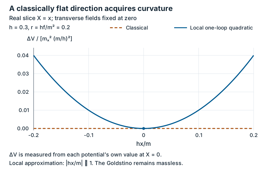
Along the real slice $X=x$ with both transverse scalars fixed at zero, the classical valley is flat. The solid curve shows the local quadratic rise from the quantum potential’s value at $X=0$; the dashed curve is measured from the classical potential’s own value there. The positive curvature gives the scalar a mass while the Goldstino remains massless. This illustrates the local approximation for the stated $r=0.2$, weak-coupling example, rather than the full potential.

Our classical bound was global. The quantum calculation here establishes a local minimum and its curvature; it has not analyzed the effective potential at arbitrarily large $X$ or specified an ultraviolet completion. Nor does “nonsupersymmetric” automatically mean “metastable”: a decay claim requires a lower region and a barrier, and a lifetime requires additional work.

Exercises

1. Locate the threshold and identify the missing light field

Keep $f,h,m>0$ and examine $X=\phi_2=0$, $\phi_1=ib/\sqrt2$ with real $b$. Derive the potential along this line. What happens at $r=1$ and at $r>1$? Does the continued nonzero $F_X$ at the origin make that point a stable broken vacuum?

Hint 1

Keep the quartic term when the quadratic coefficient vanishes.

Hint 2

The Goldstino argument is about a broken symmetry at a vacuum. A zero fermion mass at an unstable stationary configuration is not a stability proof.

Solution

On this line $W_X=f-hb^2/4$ and $|W_2|^2=m^2b^2/2$, giving

$$V(b)=f^2+\frac12(m^2-hf)b^2+\frac{h^2}{16}b^4.$$

For $r<1$ the origin has positive curvature along $b$. At $r=1$ the quadratic term vanishes, but the quartic is positive: this direction is not an exactly flat classical modulus. It is an additional massless fluctuation at quadratic order, so a low-energy theory that had integrated it out needs to be reconsidered.

For $r>1$, arbitrarily small nonzero $b$ lowers the potential. The origin is a saddle, despite $F_X=-f$ and the massless $\psi_X$ there. The nonzero minima on this particular line occur at

$$b^2=\frac{4(hf-m^2)}{h^2}.$$

Finding these line minima alone does not classify the full new vacuum set. The strict stable regime used in the lesson cannot be extended by ignoring the negative eigenvalue or by analytically continuing a determinant through it.

2. Show positivity without a numerical approximation

Let $N(r)=(1+r)^2\log(1+r)-(1-r)^2\log(1-r)-2r$. Use $N'''(r)$ to obtain a positive power series for $\nu(r)=N(r)/r^3$ on $0<r<1$. Recover the first two terms and explain why the result gives the mass of both real components of $X$.

Hint 1

$N(0)=N'(0)=N''(0)=0$. Expand $1/(1-r^2)$ and integrate three times.

Hint 2

The potential contains $m_X^2|X|^2$, while the real-field kinetic terms each carry $1/2$.

Solution

Differentiation gives $N'''(r)=4/(1-r^2)$. The three vanishing initial values fix all integration constants. Termwise integration of the convergent geometric series gives

$$N(r)=\sum_{n=0}^\infty \frac{4r^{2n+3}}{(2n+1)(2n+2)(2n+3)}.$$

Therefore

$$\nu(r)=\sum_{n=0}^\infty \frac{4r^{2n}}{(2n+1)(2n+2)(2n+3)} =\frac23+\frac{r^2}{15}+\frac{2r^4}{105}+\cdots.$$

Every coefficient is positive. This supplies an analytic positivity check independent of evaluating the logarithms at sample points. Multiplying by $h^2m^2r^2/(32\pi^2)$ gives the leading mass $h^4f^2/(48\pi^2m^2)$.

Finally $|X|^2=(X_R^2+X_I^2)/2$ and $|\partial X|^2=[(\partial X_R)^2+(\partial X_I)^2]/2$. The same coefficient $m_X^2$ is therefore the mass squared of each canonically normalized real component. Neither real scalar is required to remain degenerate with the Goldstino in this broken vacuum.

3. A small interaction can create distant supersymmetric vacua

Modify the superpotential by $\Delta W=\varepsilon m\phi_2^2/2$, with fixed real $\varepsilon\ne0$. Solve all F equations. Where do the solutions go as $\varepsilon\to0$? Does the existence of those solutions, together with our undeformed one-loop mass, calculate a metastable lifetime?

Hint 1

The equation for $\phi_2$ first gives $\phi_2=-\phi_1/\varepsilon$. The $X$ equation ensures $\phi_1\ne0$.

Hint 2

A fixed superpotential coefficient can break R symmetry while preserving supersymmetry of the action. The new theory requires its own local stability calculation.

Solution

The equations are

$$f+\frac h2\phi_1^2=0,\qquad hX\phi_1+m\phi_2=0,\qquad m\phi_1+\varepsilon m\phi_2=0.$$

The first gives $\phi_1=\pm i\sqrt{2f/h}$. The other two then imply

$$X=\frac{m}{h\varepsilon},\qquad \phi_2=-\frac{\phi_1}{\varepsilon}.$$

All three auxiliaries vanish, so both solutions have zero energy with canonical kinetic terms. This agrees with Intriligator–Seiberg, §2.6, (2.36)–(2.39). As $\varepsilon\to0$, $X$ and $\phi_2$ escape to infinity; no finite supersymmetric solution of the original model is recovered.

The deformation preserves supersymmetry of the action. With $\varepsilon$ fixed and neutral, its operator has R-charge four instead of the required two, so it explicitly breaks the selected R symmetry.

The lower-energy supersymmetric solutions change the global question, but the undeformed curvature is not the effective potential of the new theory. To establish a nearby metastable state, recompute its stationary point and transverse stability with the deformation included. To calculate its lifetime, determine the barrier and a tunneling solution in a controlled regime. The F roots alone provide neither calculation.

The model now separates three statements that are easy to conflate: incompatible F equations exclude a supersymmetric configuration, the classical bound establishes stable minima, and the loop determinant lifts their scalar degeneracy. The Goldstino follows the broken global symmetry through that last step.