ABJM large N and the Airy approximation

Two curves can overlap on a free-energy plot while disagreeing by much more than the numerical error. Conversely, a tiny difference can be entirely numerical. This laboratory makes both situations visible. Starting from the positive ABJM density kernel, you will calculate finite-rank partition functions, plot $F/N^{3/2}$, and then magnify the discrepancy from the perturbative Airy answer.

Read the Airy function and the corrections it omits first. Its determinant and asymptotic derivations supply our analytic preparation; the present task is an independent finite-rank computation and its error diagnosis.

The observable and the fixed limit

We keep the undeformed three-dimensional compact $U(N)_k\times U(N)_{-k}$ theory, with rank $N$ per factor and no further quotient. All variables below are dimensionless. The round-sphere measure and positive first-node Chern–Simons phase are fixed as in the prerequisite. There are no real masses or FI sources. The generic theory has twelve real Poincaré supercharges, enhanced to sixteen at the two levels used here, $k=1,2$; this full-theory count differs from the chosen supercharge used in the manifest $\mathcal N=2$ localization calculation.

The physical observable is $Z_N=Z_{S^3}(N,k)>0$, with $F_N=-\log Z_N$. The auxiliary Fermi gas is ungraded, and $Z_N$ is not an index. Increasing $N$ at fixed positive $k$ tests the M-theory large-rank limit. It is not the ’t Hooft limit, which increases $N,k$ together at fixed $\lambda=N/k$.

On $L^2(\mathbb R,dx)$, use

$$\rho_k(x,y)=\frac{1}{8\pi k\sqrt{\cosh(x/2)\cosh(y/2)} \cosh[(x-y)/(2k)]},\qquad \operatorname{Tr}\rho_k=\frac1{4k}. \tag{LAB11.1}$$

The factor $dx$, rather than $dx/(2\pi)$, matters in this expression. Its operator is positive and trace class. If its eigenvalues are $\lambda_j\geq0$, the Fermi-gas formulation gives

$$\det(1+z\rho_k)=\prod_j(1+z\lambda_j) =\sum_{N=0}^\infty Z_Nz^N,\qquad Z_0=1. \tag{LAB11.2}$$

Here $z$ is an auxiliary fugacity, not a mass. The kernel and determinant follow FG (3.3) and (3.24). We compute the coefficients of this full determinant numerically; the Airy function is not used to generate those data.

A positive coefficient calculation

Replace the real line by $[-L,L]$. Let $x_i,w_i$ be the nodes and positive weights of an $n$-point Gauss–Legendre quadrature on that interval. The symmetric weighted matrix is

$$K_{ij}=\sqrt{w_iw_j}\,\rho_k(x_i,x_j). \tag{LAB11.3}$$

Diagonalizing $K$ approximates the integral-operator spectrum. It does not make the integral discretization exact. If $c_m$ is the coefficient of $z^m$ after some eigenvalues have been included, adding one more eigenvalue $\lambda$ gives

$$c_m^{\rm new}=c_m^{\rm old}+\lambda c_{m-1}^{\rm old}, \qquad c_0=1. \tag{LAB11.4}$$

The two terms choose whether to occupy that level. Both use the old array; updating upward in place would reuse the same fermionic level. Every addition is positive, so this method avoids alternating Newton identities between nearly equal traces. The program actually stores $\log c_m$ and uses a stable log-sum operation. This also prevents underflow of small $Z_N$.

Exact positivity does not prevent tiny negative eigenvalues in floating-point arithmetic. The program records their total absolute size $s_-$, rejects an eigenvalue below $-2\times10^{-14}$, and otherwise omits only those negative values. This numerical threshold is a diagnostic choice, not a physical cutoff. Small positive eigenvalues can also contain error; recording $s_-$ alone cannot certify them.

Mathematical input	Program name	Meaning
$k,N_{\max}$	k, nmax	Fixed level and largest requested rank
$L,n$	L, nodes	Independent window and quadrature controls
$\log Z_N$	log_Z	Positive coefficient recursion
$F_N-F_N^{\rm pert}$	F_minus_F_pert	Signed free-energy discrepancy
$s_-$	negative_eigenvalue_mass	Recorded floating-point sign defect

The two predictions

The leading prediction is $F_N/N^{3/2}\to a_k=\pi\sqrt{2k}/3$. The normalized perturbative prediction is

$$Z_N^{\rm pert}=e^{A(k)}C^{-1/3}\operatorname{Ai}[C^{-1/3}(N-B)], \quad C=\frac2{\pi^2k},\quad B=\frac{k}{24}+\frac1{3k}, \tag{LAB11.5}$$ $$A(1)=\frac{\log2}{4}-\frac{\zeta(3)}{8\pi^2},\qquad A(2)=-\frac{\zeta(3)}{2\pi^2}. \tag{LAB11.6}$$

These special values use the constant-map prescription of HMO (3.4), identified there as a conjectured input tested with exact data. They are not fitted to the kernel calculation. The prerequisite explains the prescription and the cubic inversion; HMO (3.18) gives the resulting Airy expression. The script deliberately supports only $k=1,2$, where these absolute constants are supplied.

The exact Fredholm determinant is periodic in a chemical potential $\mu$ through $z=e^\mu$; $\exp(C\mu^3/3+B\mu+A)$ is a perturbative branch, not that exact determinant. Its Airy coefficient resums algebraic large-$N$ corrections but omits exponential sectors. Quantify the omission with the signed ratio used in HMO (1.6):

$$\delta_N=\frac{Z_N}{Z_N^{\rm pert}}-1, \qquad F_N-F_N^{\rm pert}=-\log(1+\delta_N). \tag{LAB11.7}$$

Evaluating this as expm1(log_Z - log_Z_pert) avoids a second loss of significant digits. It cannot recover digits already lost in the kernel calculation.

Run and read the comparison

Save these four files in one directory:

Download the complete lab (ZIP) with the program, pinned dependencies, reference output and run instructions.

• Standalone Python calculation.
• Pinned dependencies.
• Expected default physical values and tolerance.
• Reproducible two-panel figure.

The tested environment is Python 3.13.7, NumPy 2.1.2 and mpmath 1.3.0. In a fresh environment, install the dependencies and run:

python -m pip install -r requirements.txt
python large_n.py --json result.json --svg large_n.svg --check-expected expected-output.json
python large_n.py --k 1 --nmax 12 --json level-one.json
python large_n.py --k 1 --coarse --json coarse.json

The default is $k=2$, $N=1,\ldots,8$. Four calculations use every combination $L=80,96$ and $n=768,1024$. The final value is from $(96,1024)$. The deliberately coarse option instead uses $L=48,64$ and $n=128,192$; it is a negative control. The script makes no network calls and does not import another laboratory. --dps changes the Airy and source-constant working precision, not the NumPy kernel, which remains double precision.

Representative default values are:

$N$	$F_N/N^{3/2}$	$\delta_N$	Empirical indicator in $F$
1	2.0794415417	$2.5194518\times10^{-3}$	about $4\times10^{-13}$
2	2.0347689442	$4.3144100\times10^{-4}$	about $7\times10^{-13}$
4	2.0372565548	$2.5701789\times10^{-5}$	about $1.4\times10^{-12}$
8	2.0530069131	$3.3242323\times10^{-7}$	about $3.2\times10^{-12}$

Last digits of the diagnostic columns depend on the linear-algebra platform. The expected-output file compares physical columns with an absolute tolerance of $5\times10^{-11}$; it does not demand identical roundoff.

The upper panel compares one observable in the same normalization. The lower panel shows the magnitude of its signed residual; plus or minus labels retain its sign. Open symbols mean the empirical indicator does not resolve the residual. The dotted indicator is not a certified error bar. A short sequence of ranks illustrates convergence; it does not establish an asymptotic theorem.

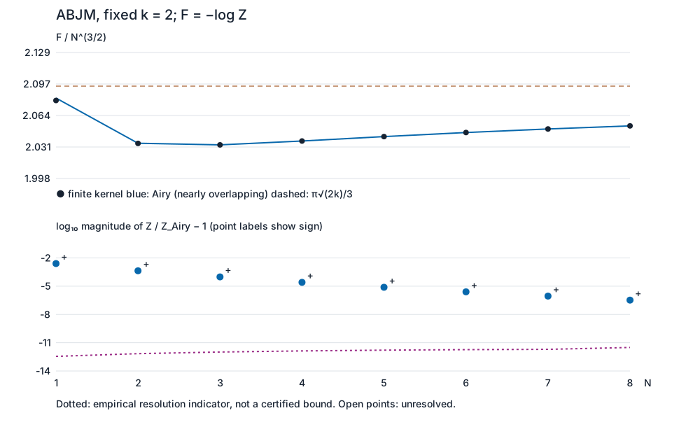
The leading constant for this plot is $2\pi/3\simeq2.0943951$. Its visible finite-rank bias is much larger than the Airy discrepancy. Thus leading scaling, perturbative resummation and full finite-rank data answer three different accuracy questions.

What the checks actually bound

An analytic fact controls the lost diagonal trace outside the window:

$$t_L=\operatorname{Tr}\rho-\operatorname{Tr}(P_L\rho P_L) =\frac{\arctan(e^{-L/2})}{\pi k}. \tag{LAB11.8}$$

Here $P_L$ restricts wavefunctions to $[-L,L]$. For the exact compressed operator, let $Z_m^L$ be its determinant coefficients. Ordered eigenvalues obey $\lambda_j\geq\mu_j\geq0$ by the variational principle, with $\sum_j(\lambda_j-\mu_j)=t_L$. Expanding each coefficient in $\mu_j$ and $d_j=\lambda_j-\mu_j$, then allowing overlapping selections to overcount, gives

$$0\leq Z_N-Z_N^L \leq\sum_{j=1}^N\frac{t_L^j}{j!}Z_{N-j}^L. \tag{LAB11.9}$$

We used $e_j(d)\leq(\sum d)^j/j!$ for nonnegative numbers. This is a genuine operator-compression bound. In the program its right side is evaluated with numerical $Z_m^L$: that evaluation is not a bound on quadrature or diagonalization error. The exact mathematical statement and the numerical substitution must remain separate.

For an empirical resolution indicator, the program takes ten times the largest observed change in $F$ on either axis of the four-run grid, the sensitivity scale $s_-Z_{N-1}/Z_N$, and a floating-point floor $32N\epsilon_{\rm mach}$; it then adds the logarithmic version of (LAB11.9). The factor ten is a declared conservative convention, not a confidence level or a theorem. The JSON report exposes every contribution. Agreement on this grid is useful evidence, but errors common to all four grids can survive it.

Independent calibration catches some such errors. HMO Appendix B gives, for example,

$$Z_1(k=2)=\frac18,\quad Z_2(k=2)=\frac1{32\pi^2},\quad Z_4(k=2)=\frac{24-32\pi^2+3\pi^4}{49152\pi^4}. \tag{LAB11.10}$$

The script compares these values, and their $k=1$ counterparts, with the kernel output. Checks through $N=8$ against additional source formulas had relative differences below $2\times10^{-13}$ in the tested environment. A separate positive real Bessel integral also reproduced the normalized Airy values. Neither check makes all future higher-rank coefficients exact.

At fixed $k$, the omitted sectors have actions proportional to $\mu_*$ or $\mu_*/k$, where $\mu_*\sim\sqrt{N/C}$. Their coefficients and cancellations matter: at $k=1$ the leading combined correction is much smaller than at $k=2$. The optional $k=1,N=12$ result is unresolved by this calculation. Increasing --dps alone does not change that. On a fixed-$\lambda$ path, these scales and $B/N$ behave differently; this laboratory does not convert its fixed-level evidence into uniform ’t Hooft error control.

Exercises

1. Change the density normalization

A copied measure accidentally multiplies the kernel by $s=1.001$. Derive the change in $F_N/N^{3/2}$ and in $\delta_N$, holding the intended Airy normalization fixed. Estimate the error at $N=8$. Which independent check catches it?

Hint 1. Each term of the $N$th coefficient contains exactly $N$ eigenvalues.

Hint 2. Compare $s^NZ_N$ with the same $Z_N^{\rm pert}$, not with a refitted $A$.

Solution

Every eigenvalue is multiplied by $s$, so $Z_N\mapsto s^NZ_N$ and $F_N\mapsto F_N-N\log s$. The normalized change is $-\log s/\sqrt N$, about $-3.5338\times10^{-4}$ at $N=8$. Also $\delta_N\mapsto s^N(1+\delta_N)-1$, about $0.0080284$ for the default $N=8$ value, overwhelmingly larger than $3.324\times10^{-7}$. The trace becomes $s/(4k)$, so even the $N=1$ calibration detects the wrong measure. A constant adjustment of $A$ cannot remove an error proportional to $N$ at every rank. Positive eigenvalues and stable quadrature would not detect this convention error by themselves.

2. Explain the leading plot’s bias

Use the large-positive-argument Airy asymptotic $\operatorname{Ai}(x)\sim e^{-2x^{3/2}/3}/(2\sqrt\pi x^{1/4})$ to derive the first corrections to $F_N^{\rm pert}/N^{3/2}$. What happens to $B/N$ if $k=N/\lambda$ instead of being fixed?

Hint 1. Keep the prefactor $e^AC^{-1/3}$ before expanding $N-B$.

Hint 2. Expand $(N-B)^{3/2}$ at fixed $B$ first; only afterward inspect whether this ordering survives the changed path.

Solution

Taking the negative logarithm gives

$$F_N^{\rm pert}=\frac{2(N-B)^{3/2}}{3\sqrt C} +\frac14\log(N-B)+\log(2\sqrt\pi)+\frac14\log C-A +O(N^{-3/2}).$$

At fixed $k$, division by $N^{3/2}$ therefore yields

$$\frac{F_N^{\rm pert}}{N^{3/2}} =a_k-\frac{B}{\sqrt C\,N} +\frac{\tfrac14\log N+\log(2\sqrt\pi)+\tfrac14\log C-A}{N^{3/2}} +O(N^{-2}).$$

For $k=2$, $B=1/4$, $1/\sqrt C=\pi$, so the leading normalized bias is $-\pi/(4N)$. The next displayed term partly offsets it. These power corrections explain why the upper plot’s discrepancy from $2\pi/3$ is far larger than its Airy residual. On $k=N/\lambda$, however, $B/N=1/(24\lambda)+\lambda/(3N^2)$ does not tend to zero; $C$ and $A(k)$ also change. The fixed-$k$ expansion is not a uniform expansion along that path. An integer-level sequence with a specified rational $\lambda$ can realize the path, but it poses a different asymptotic problem.

3. Diagnose an apparent negative correction

Run python large_n.py --k 1 --coarse. Near $N=4$, the program returns $\delta_4\simeq-1.05\times10^{-5}$, whereas the refined calculation gives about $+1.05\times10^{-8}$. Explain which evidence rejects the coarse sign. Then interpret a $k=1,N=12$ residual of order $10^{-13}$ with an indicator of order $4\times10^{-12}$.

Hint 1. Compare the change in $F$ under node refinement with $-\log(1+\delta_N)$.

Hint 2. Check the independent exact $Z_4$ before assigning the discrepancy to an omitted instanton sector.

Solution

The coarse $N=4$ free-energy discrepancy is only about $10^{-5}$, while its node change is about $0.0031$ and its empirical indicator about $0.031$. Its exact-source relative calibration error is itself about $10^{-5}$. The sign is a discretization artifact in this test, as the refined source-calibrated value confirms. It is not evidence for a negative physical sector.

At $k=1,N=12$, the residual lies below the observed resolution scale. Report it as unresolved; neither its sign nor agreement with zero is meaningful at that precision. More Airy digits do not repair the double-precision eigensystem. A further investigation would need a better-conditioned or higher-precision spectral representation, independent refinement and a renewed error budget. It must not set the physical correction to zero simply because this implementation cannot see it.

The useful outcome is a comparison with three explicit scales: the leading finite-rank bias, the much smaller Airy omission, and the numerical resolution. Keep those scales separate when moving to a more demanding rank or level.