Hopf fibers and transverse geometry

A circle drawn on a sphere is not automatically a fiber, and a closed curve on the base need not lift to a closed horizontal curve. This laboratory makes both distinctions calculable. You will draw two fibers, check the geometry without choosing local coordinates, and transport a point around a base loop that passes through the missing pole of a familiar section.

Prepare with circle bundles and the Hopf fibration and almost contact metric structures. Those lessons supply the analytic construction and its geometric meaning. Here we turn their formulas into a portable calculation, including tests that fail when a component is omitted.

Fix the circle action before computing

Write a point of the unit three-sphere as $y=(y_0,y_1,y_2,y_3)$, with $y^Ty=1$, and assemble two complex coordinates $z_1=y_0+iy_1$, $z_2=y_2+iy_3$. The column $z$ is not a supersymmetry parameter. The physical round metric is $g=\ell^2dy^Tdy$ on tangent vectors, with radius $\ell>0$.

The Hopf map and the circle action are

$$n=(2\operatorname{Re}\bar z_1z_2,\;2\operatorname{Im}\bar z_1z_2, |z_1|^2-|z_2|^2),\qquad z\longmapsto e^{i\chi}z,\qquad \chi\sim\chi+2\pi. \tag{LAB05.1}$$

Every orbit lies over one point $n\in S^2$. Increasing $\chi$ fixes its orientation. We orient $S^3$ as the outward boundary of the unit ball in the ordered real coordinates $(y_0,y_1,y_2,y_3)$, and $S^2$ outward in its three $n$ coordinates.

The normalized principal connection is

$$\Theta=-iz^\dagger dz =y_0dy_1-y_1dy_0+y_2dy_3-y_3dy_2, \qquad \Theta(\xi_0)=1, \quad \xi_0=(-y_1,y_0,-y_3,y_2). \tag{LAB05.2}$$

The metric-unit objects are instead $\eta=\ell\Theta$ and $\xi=\xi_0/\ell$. A fiber has circumference $2\pi\ell$. In P (5.11), the round limit has $r=\ell$, $h=1$ and the paper’s angular coordinate has period $4\pi$: locally $\psi=2\chi_N$, and the paper’s connection bracket is $2\Theta$. Missing this factor changes both the metric and the apparent bundle number.

This is a calculation in three-dimensional positive metric geometry. We choose no supergravity sources or dynamical gauge theory, so no preserved supercharge count or gauge rank is assigned by the laboratory.

Check the integer before plotting

Use northern and southern sections

$$s_N=\begin{pmatrix}\cos(\theta/2)\\e^{i\phi}\sin(\theta/2)\end{pmatrix}, \qquad s_S=\begin{pmatrix}e^{-i\phi}\cos(\theta/2)\\\sin(\theta/2)\end{pmatrix}. \tag{LAB05.3}$$

They obey $s_N=e^{i\phi}s_S$. For the same total-space point, therefore, $\chi_S=\chi_N+\phi$ modulo $2\pi$. Pulling back (LAB05.2) gives

$$\Theta=d\chi_N+\frac{1-\cos\theta}{2}d\phi =d\chi_S-\frac{1+\cos\theta}{2}d\phi, \qquad \mathcal F=d\Theta=\frac{\sin\theta}{2}d\theta\wedge d\phi. \tag{LAB05.4}$$

Here the curvature on the right is understood as a form on the base and then pulled back. Its integral is exactly $\int_{S^2}\mathcal F=2\pi$, so the first Chern number is $+1$. The transition function has the same unit winding. The program integrates this formula symbolically; it does not infer an integer by rounding a sampled flux.

The two sections are useful, but neither covers the entire base. The coordinate column $z$ in the ambient $\mathbb C^2$ description has no such local-section singularity.

Test the whole transverse tensor

Let $J_0$ denote multiplication by $i$ on both complex coordinates: $J_0y=\xi_0$. Define the tangent and horizontal projectors

$$\Pi=I_4-yy^T,\qquad \Pi_h=\Pi-\xi_0\xi_0^T, \qquad \Phi=-J_0\Pi_h. \tag{LAB05.5}$$

“Horizontal” means annihilated by $\Theta$. At $y=(1,0,0,0)$ the oriented tangent basis is $(E_1,E_2,E_3)$, with $E_j$ in the $y_j$ direction. Thus $\Phi E_2=-E_3$ and $\Phi E_3=E_2$, precisely the convention of the prerequisite lesson.

Because $J_0^2=-I_4$ and $J_0$ preserves the horizontal plane, multiplication gives

$$\Phi^2=-\Pi_h,\quad \Phi\xi_0=0,\quad \xi_0^T\Phi=0,\quad \Phi^T\Phi=\Pi_h. \tag{LAB05.6}$$

Restricted to the tangent space, these are P (B.1)–(B.2), including metric compatibility. The radial direction is an extra zero direction of our ambient four-by-four matrix, not an extra tangent direction on $S^3$.

The script also differentiates the Hopf map itself. For a horizontal tangent vector $X$ it finds $|dn(X)|^2=4|X|^2$, confirming the base radius $\ell/2$. Finally, the circle flow $R_\chi=e^{\chi J_0}$ obeys

$$\Phi(R_\chi y)=R_\chi\Phi(y)R_\chi^{-1}. \tag{LAB05.7}$$

This says that the transverse rotation is preserved along fibers. Its infinitesimal version is the full tensor Lie derivative $\mathcal L_{\xi_0}\Phi=0$, including the index-rotation terms. It is stronger than the projected condition in P (B.8). Meanwhile $\Theta\wedge d\Theta$ never vanishes: the horizontal planes are not tangent to surfaces. A transverse complex structure on the base and nonintegrable horizontal planes are compatible statements.

Draw actual fibers

Choose the two base points $n=(\pm1,0,0)$ and their lifts $z=(1,\pm1)/\sqrt2$. Their fibers are the literal curves $e^{i\chi}(1,\pm1)/\sqrt2$. The script projects them to $\mathbb R^3$ by

$$\boldsymbol r=\frac{(-y_1,y_2,y_3)}{1-y_0}. \tag{LAB05.8}$$

The omitted point is $(1,0,0,0)$, which belongs to neither displayed fiber. The minus sign makes this chart preserve the declared outward orientation. The resulting circles have centers $(0,\pm1,0)$, radius $\sqrt2$, and planes $r_3=\mp r_1$.

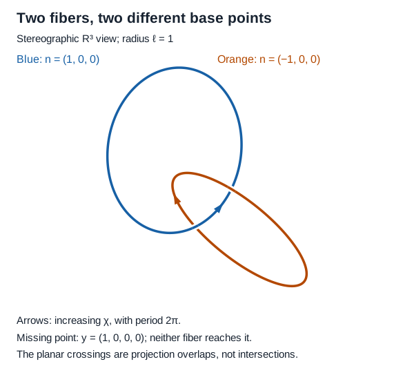
The view is a fixed orthographic projection of those three-dimensional circles, at $\ell=1$. Its apparent crossings are not intersections of fibers. Distances in the picture are not round-sphere distances. Both circles close at $\chi=2\pi$ and have linking number $+1$ with the declared orientations. One can establish the sign without a plot: the second circle pierces the oriented planar disk of the first once positively. A separate Gauss linking integral checks the numerical parametrization.

Lift a loop that crosses a section’s missing point

Let $c\in(-1,1)$ be a latitude cosine and set $s=\sqrt{1-c^2}$. Use the oriented orthonormal triple

$$a=(s,0,-c),\quad b=(c,0,s),\quad d=a\times b=(0,-1,0), \qquad n(t)=ca+s(b\cos t+d\sin t),\quad 0\le t\le2\pi. \tag{LAB05.9}$$

This tilted latitude passes through the south pole at $t=\pi$. Its cap about the axis $a$ has positive area $2\pi(1-c)$ on the unit base sphere, hence curvature flux $\pi(1-c)$.

For transport, use the ordinary Pauli matrices $\sigma=(\sigma_1,\sigma_2,\sigma_3)$ with $\sigma_3=\operatorname{diag}(1,-1)$. They encode the coordinate identity $z^\dagger\sigma z=n$; they are not a change to the site’s spacetime gamma-matrix convention. The rank-one projector onto the coordinate line is $P_n=(I_2+n\cdot\sigma)/2$. A globally regular horizontal-lift equation is

$$\dot z=\dot P_n z=\frac12\dot n\cdot\sigma\,z, \qquad z(0)=\begin{pmatrix}s\\c\end{pmatrix}. \tag{LAB05.10}$$

To see why this works, differentiate $P_n^2=P_n$ to get $P_n\dot P_nP_n=0$. On $P_nz=z$, (LAB05.10) preserves that constraint and gives $z^\dagger\dot z=0$, preserving the norm and imposing $\Theta(\dot z)=0$. All coefficients stay smooth at $t=\pi$.

There is also a check that does not integrate this equation numerically. Rotating about $a$ gives $U(t)=\cos(t/2)I_2-i\sin(t/2)a\cdot\sigma$. Its lift has $z^\dagger\dot z=-ic/2$, so multiplication by a compensating phase gives

$$z_H(t)=e^{ict/2}U(t)z(0),\qquad z_H(2\pi)=e^{-i\pi(1-c)}z(0). \tag{LAB05.11}$$

The return phase agrees with $e^{-i\int\mathcal F}$. It is the phase of a horizontally transported point in the bundle. A charge-$m$ field component with convention $D=d-ima$ has the opposite-sign parallel-transport phase $e^{+im\oint a}$; do not interchange these objects.

For the default $c=1/2$, the return phase is $-i$. The base closes once while its horizontal lift does not. This is different from the fibers drawn above, whose base point never moves.

Reproduce and read the result

Download the complete lab (ZIP) with the program, pinned dependencies, reference output and run instructions.

Download the Python script, pinned requirements, expected output, and the reproducible SVG into one directory. The tested environment is Python 3.13.7, SymPy 1.13.3 and mpmath 1.3.0. No plotting package, network access, or site checkout is needed after installation.

python -m pip install -r requirements.txt
python hopf_fibration.py
python hopf_fibration.py --figure hopf-fibers.svg
python hopf_fibration.py --cosine 1/3

Mathematical object	Variable or function	What it checks
$J_0,\Pi,\Pi_h,\Phi$	J, P, H, Phi in exact_checks	Exact identities modulo $y^Ty=1$; H here is a projector, not a supergravity source
$n,\dot n,z_H$	base, velocity, exact in data	Smooth loop and an analytic reference curve
(LAB05.10)	rhs inside integrate	Four-stage Runge–Kutta transport
(LAB05.8)	point inside figure	Native SVG generated from the actual fibers

The default run passes 23 grouped exact assertions. The transport uses 50 decimal digits and does not renormalize after steps, so norm drift remains observable. The maximum vector error over all step endpoints is

Steps around the loop	Maximum vector error	Maximum norm-squared drift
64	$2.61152\times10^{-7}$	$4.54939\times10^{-7}$
128	$1.61382\times10^{-8}$	$2.80134\times10^{-8}$
256	$1.00294\times10^{-9}$	$1.73771\times10^{-9}$

The error ratios are $16.18$ and $16.09$, approaching the factor $2^4$ expected for fourth-order global error. More decimal digits alone do not remove the finite-step error. The tiny approximately $10^{-52}$ real part in the printed exact $-i$ phase is rounding; it is not a geometric correction. The displayed error is measured at step endpoints, not a certified continuous-time bound.

The exact tensor tests, analytic cap flux and rotating-frame solution address different possible errors. A further check replaces the loop by short geodesic edges, transports by successive normalized projectors $P_{n_{j+1}}$, and compares with the polygon’s oriented solid angle. That method converges to the same smooth-loop phase at second order, rather than fourth: it approximates a different curve at finite resolution.

Exercises

1. A transverse test that misses a vertical error

At $y=(1,0,0,0)$, let $u=E_2$ and change the tensor to $\Phi_\varepsilon=\Phi+\varepsilon\xi_0u^T$. Does testing only $\Pi_h\Phi_\varepsilon\Pi_h$ detect the error? Evaluate the full vertical and norm tests for $\varepsilon=1/3$. What would you add to a test suite?

Hint 1

The added output points along $\xi_0$, which the left horizontal projector removes.

Hint 2

Apply the modified tensor to $u$. Compare both its $\Theta$ component and its squared length with the required values.

Solution

Since $\Pi_h\xi_0=0$, the projected test gives exactly $\Pi_h\Phi_\varepsilon\Pi_h=\Phi$ for every $\varepsilon$. But

$$\Phi_\varepsilon u=-E_3+\varepsilon E_1,\qquad \Theta(\Phi_\varepsilon u)=\varepsilon,\qquad |\Phi_\varepsilon u|^2=1+\varepsilon^2.$$

At $\varepsilon=1/3$ the last two results are $1/3$ and $10/9$, instead of zero and one. The modified tensor fails to map horizontal vectors into horizontal vectors and fails metric compatibility. Test the full left kernel $\Theta\Phi=0$ and $\Phi^T\Phi=\Pi_h$, in addition to projected identities. The released script includes this negative control: its successful projected check is deliberately insufficient.

2. Repair the local section at the pole

For the default $c=1/2$, show that the north section has different limiting values as the loop approaches $t=\pi$ from either side, although $z_H(t)$ is smooth. Give the limiting azimuths and show how the transition to $s_S$ removes the discrepancy. Is this a change of the connection or of its description?

Hint 1

Near $t=\pi$, use $n_1=\sqrt3(1+\cos t)/4$ and $n_2=-\sqrt3\sin t/2$.

Hint 2

At the south pole the north section tends to $(0,e^{i\phi})$, whereas the south section tends to $(0,1)$. Remember $\chi_S=\chi_N+\phi$.

Solution

Writing $t=\pi+\delta$, we have $n_1=\sqrt3\delta^2/8+O(\delta^4)$ and $n_2=\sqrt3\delta/2+O(\delta^3)$. Thus the azimuth tends to $-\pi/2$ on approach and $+\pi/2$ on departure. The north section tends to $(0,-i)$ and $(0,+i)$: the two local representatives differ by a sign.

The exact lift is finite and smooth. Direct substitution in (LAB05.11) gives $z_H(\pi)=(0,e^{-i\pi/4})$. Its north fiber coordinate compensates for the changing section. In the south description, $s_S\to(0,1)$ and $e^{i\chi_S}\to e^{-i\pi/4}$ on both sides, because $\chi_S=\chi_N+\phi$. The local potentials differ by $a_N-a_S=d\phi$, while $d\chi_N+a_N=d\chi_S+a_S$. The global connection is unchanged. An algorithm that treats the north section’s jump as a jump of the transported point has confused a coordinate representative with the point itself.

3. When does a horizontal lift close?

Change the latitude cosine to $c=1/3$ and run the final command above. Predict the return phase and the least number of complete base circuits needed to close the horizontal lift. Compare with the default. What happens for irrational $c$? Determine the length of the closed default lift and compare it with a single Hopf fiber.

Hint 1

After $q$ repetitions, the accumulated phase is $e^{-iq\pi(1-c)}$. Ask when this is one.

Hint 2

The base radius is $\ell/2$. A horizontal lift has the same length as its base curve in that metric; a single latitude circuit has length $\pi\ell\sqrt{1-c^2}$.

Solution

For $c=1/3$ the phase is $e^{-2\pi i/3}=-1/2-i\sqrt3/2$, so three circuits close the lift. At $c=1/2$ the phase is $-i$ and four circuits are required. In general the condition is $q(1-c)\in2\mathbb Z$; irrational $c$ admits no positive integer $q$. This is an exact arithmetic condition, not a numerical decision based on a phase close to one.

The default one-circuit length is $\pi\sqrt3\ell/2$, so its four-circuit closed lift has length $2\pi\sqrt3\ell$. A Hopf fiber has length $2\pi\ell$ and projects to a point. The longer closed horizontal curve projects to a moving latitude four times. Closing a curve does not make it a fiber, and changing this loop does not change the bundle number.

The useful outcome is a distinction among global geometry, local descriptions and numerical representations. The smooth fibers and horizontal lift are global; the local section omits a pole; the finite-step trajectory approximates a differentially defined curve. These are separate facts, and the checks should keep them separate.